How Large Language Models Work: A Guide for the Curious Techie

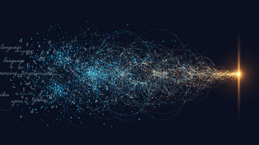
The article explains in detail how large language models (LLMs) work — from text tokenization through embedding vectors and the transformer architecture with its self-attention mechanism, all the way to response generation and the training process. Using Meta's open-source Llama 3.1 model as an example, it describes key concepts such as BPE tokenization, Grouped-Query Attention, the KV cache, weight quantization, and the Mixture of Experts architecture, all in an accessible form for IT professionals without a background in machine learning.

You type the word "Hi" into ChatGPT or Claude, and a few seconds later you get a reply. Fluent, grammatically correct, often surprisingly clever. But behind that reply lies a chain of operations that begins by breaking your text into pieces, continues with the multiplication of enormous matrices, and ends with a probabilistic guess at the next word. No magic, no consciousness — just linear algebra at industrial scale.

This article explains how large language models (LLMs) work, step by step. You don't need to know machine learning for it; basic IT literacy and a willingness to think about numbers are enough. As our reference model we use Meta's Llama 3.1 — it is open-source, its architecture is publicly documented, and by design it is representative of most of today's LLMs, including ChatGPT and Claude.

Why is it useful to understand the mechanism, not just the results? Because someone who grasps how a model "thinks" can better judge when to trust it and when not to. They will understand why Czech costs more on the API than English, why a model occasionally "hallucinates," and why the answer to the same question is a little different every time.

A language model does not work with letters or with words. It works with tokens — pieces of text that are a compromise between characters and whole words.

Processing text character by character would be too slow — a twenty-word sentence would have tens to hundreds of positions, and the model would have to infer from each character which word it belongs to. Processing whole words, on the other hand, would require an enormous vocabulary: Czech, with its declension, conjugation and prefixes, generates hundreds of thousands of word forms. And a typo or a new word would be completely unknown to the model.

The solution is Byte Pair Encoding (BPE) — an algorithm that automatically finds the optimal pieces of text. It first starts with individual bytes (256 possible values). Then it repeatedly finds the most frequent adjacent pair and merges it into a new token. The process repeats until the vocabulary reaches the desired size.

The result is a vocabulary in which frequent words like "the" or "je" have their own token, while rarer words are broken into subwords. For example, "tokenizace" might split into token + iz + ace.

It depends on the model. Llama 3.1 uses a vocabulary of 128,256 tokens — four times more than Llama 2 (32,000). A larger vocabulary means frequent words are encoded as a single token instead of several, which speeds up both processing and generation. GPT-4 uses roughly 100,000 tokens.

Practical impact: Czech needs roughly 30–50% more tokens for the same content than English. This directly affects the cost of API calls and how much text fits into the model's context window.

Llama 3 and newer models use a tokenizer based on tiktoken (byte-level BPE); older models and some other architectures use SentencePiece. The principle, however, is the same.

A token itself is just a number — an identifier in the vocabulary. The token "pes" (dog) might have ID 4821, say. But the model needs to work with the meaning of words, not just with their serial number.

That is why each token ID is converted into an embedding — a dense vector of real numbers with hundreds to thousands of dimensions:

"pes" → token ID: 4821 → embedding: [0.23, -1.4, 0.07, …, 0.54] (a vector of length 4096)

The embedding dimension is the key parameter that determines the "width" of the entire model. As the number of parameters grows, so does the width: Llama 3.1 8B (8 billion parameters) has an embedding of 4,096 dimensions, Llama 3.1 70B uses 8,192, and the largest Llama 3.1 405B works with 16,384 dimensions. For comparison — the older GPT-2 with 1.5 billion parameters made do with 1,600 dimensions.

These values are public for Llama, because Meta released it as open-source. For Claude or GPT-4, Anthropic and OpenAI do not publish the exact dimensions.

(Sources: Meta Llama 3.1 Technical Report; configuration files on HuggingFace.)

The values in an embedding are not designed by hand — the model learns them itself during training. But the result is remarkable: words with similar meaning have vectors that are "closer" together in space. The classic example: vector("king") − vector("man") + vector("woman") ≈ vector("queen").

The embedding table is simply a matrix of dimensions vocabulary × dimension. For Llama 3.1 8B that is 128,256 × 4,096 = over 500 million numbers for this one layer alone. And that is only the beginning.

Once we have the tokens converted into vectors, they enter the transformer — the architecture behind practically all of today's LLMs. The transformer was designed by a team at Google in 2017 (Vaswani et al., "Attention Is All You Need") and has since become the backbone of the entire field.

The transformer consists of layers (blocks) that repeat one after another. Llama 3.1 8B has 32 of them, the 405B model has 126. Each layer takes in and puts out a tensor of the same shape — the width (embedding dimension) stays constant across the whole model. Inside each layer there are two main components: self-attention and a feed-forward network.

Self-attention is a mechanism that lets each token "look at" all the other tokens and decide which are relevant to it. In the sentence "The cat sat on the mat and licked its paws," the model must understand that "licked" refers to "the cat," not to "the mat."

How does it work? From each token (a vector of dimension 4,096), a linear projection produces three vectors:

The computation then proceeds in four steps:

1. score = Q · Kᵀ # dot product — a measure of compatibility

2. score = score / √d_k # scaling (d_k = head dimension)

3. weights = softmax(score) # normalization into probabilities

4. output = weights · V # weighted sum of the values

Scaling by the square root is essential: without it, the dot products would grow with dimension and softmax would "saturate" — almost all the weight would fall on a single token and the gradients during training would be close to zero.

Instead of one large attention computation, attention is split into several heads, each working independently on a smaller dimension. For Llama 3.1 8B there are 32 heads, each of dimension 128 (32 × 128 = 4,096). Each head can specialize in a different type of relationship — one captures syntax, another pronoun coreference, yet another semantic similarity.

The outputs of all the heads are concatenated and linearly projected back onto the full dimension of 4,096.

Llama 3.1 does not use classic Multi-Head Attention, however, but Grouped-Query Attention (GQA). The difference is that while there are still 32 Query heads, there are only 8 Key and Value heads. Each group of four Q heads shares one K and V head. Why? Because K and V are stored in the KV cache (see below), and a smaller number of KV heads significantly reduces memory demands during generation — with no measurable impact on quality.

To put it in perspective: classic Multi-Head Attention with 32 KV heads takes up 4× more cache memory than GQA with 8 heads. There is also an extreme variant, Multi-Query Attention (just 1 KV head), which saves even more, but at the cost of a slight drop in quality.

(Source: Meta Llama 3.1 Technical Report, arxiv.org/abs/2407.21783)

After the attention block, each token also passes through a feed-forward network, which acts as a nonlinear transformation. Llama uses a variant called SwiGLU (instead of the classic ReLU), which has proven more efficient in practice.

The feed-forward network first expands the vector to roughly 3.5× its original width and then narrows it back down: from 4,096 to 14,336 and back to 4,096 (in Llama 3.1 8B). This expansion and contraction gives the model room for more complex transformations within each layer.

Attention by itself is a "bag of tokens" — it doesn't care about order. The sentences "the dog bit the man" and "the man bit the dog" would, without more, yield the same result. The model needs information about position.

Older models added a fixed vector to the embedding according to position (absolute positional encoding). The problem: the model generalized poorly to texts longer than those it had seen in training.

Llama and most modern models use RoPE (Rotary Position Embeddings). Instead of adding, the Q and K vectors are rotated in the complex plane according to the token's position. The key property: the dot product Q·K then depends only on the relative distance between tokens, not on absolute positions. The model naturally learns that a token two positions away has a different meaning than a token twenty positions away.

The vector is split into pairs of dimensions, and each pair is rotated at a different frequency — slow frequencies capture long distances, fast ones capture short distances. It is reminiscent of the Fourier transform. Thanks to working with relative positions, the context can be scaled by various techniques (YaRN, RoPE scaling) — which is why Llama 3.1 can handle a window of up to 128,000 tokens.

LLMs generate text autoregressively — token by token. The model receives an input sequence, computes a probability distribution over the entire vocabulary (128,256 possibilities for Llama) and selects the next token. That token is appended to the input and the whole process repeats.

This means the model does not generate the entire answer at once. Each token requires a pass through the whole network. For a model with 32 layers and vectors of 4,096 dimensions, that is an enormous amount of matrix multiplication — for every single word.

When generating the n-th token, the model needs attention over all previous tokens. Without optimization it would have to recompute the K and V vectors for the entire sequence so far — again and again, for each new token. That is needlessly expensive.

The solution: the KV cache. After the first computation, the keys and values are stored in memory and reused. A new token "queries" all the previous K's, but does not recompute them.

Token 1: compute Q₁, K₁, V₁ → store K₁, V₁

Token 2: compute Q₂, K₂, V₂ → store K₂, V₂; attention over K₁,V₁ from cache

Token 3: compute Q₃, K₃, V₃ → store K₃, V₃; attention over K₁,V₁,K₂,V₂…

How much memory does the KV cache take? For Llama 3.1 8B with GQA (8 KV heads instead of 32), it comes to roughly 128 KB per token. For 8,000 tokens that is ~1 GB, and for the maximum context of 128,000 tokens already ~16 GB — which is crucial, because the KV cache can take up more memory than the model weights themselves. This is exactly why GQA is so important: compared with classic Multi-Head Attention, it saves four times the KV-cache memory.

The model does not put out a single word, but a probability distribution over the whole vocabulary. How is a result chosen from it?

Greedy decoding always picks the token with the highest probability. It is deterministic, but often dull and repetitive. Temperature scales the logits before softmax — a lower temperature (0.1) makes the model "more certain," a higher one (1.5) more creative but also less accurate. Top-p (nucleus sampling) selects from the smallest set of tokens whose cumulative probability exceeds p (typically 0.9) — it cuts off improbable tokens but preserves diversity. Top-k simply selects from the k most probable tokens.

Most chatbots combine temperature with top-p. That is why you get a slightly different answer to the same question every time.

The model is trained on an enormous amount of text with a single task: to predict the next token. Nothing more. No instructions, no questions and answers — just raw text from the internet, books and code. And yet from such a simple task the model learns to capture surprisingly complex patterns — translation, logic, programming — without being explicitly instructed to. Whether this is genuine emergence (a sudden jump in abilities at a certain model size) or a smooth scaling effect masked by discrete metrics is a matter of lively debate (Schaeffer et al., 2023: Are Emergent Abilities a Mirage?).

input: "the dog bit" target: "the man"

The model puts out a logit vector the length of the vocabulary, and softmax turns it into probabilities. The loss function (cross-entropy) penalizes the model for assigning a low probability to the correct token. If the model assigns the token "the man" a probability of 0.42, the loss comes out to 0.87 — a relatively low penalty. If only 0.01, the loss jumps to 4.6. It is averaged over all tokens in the batch.

Backpropagation computes the gradient of the loss with respect to each weight in the model — for Llama 3.1 8B that is ~8 billion parameters. The AdamW optimizer then adaptively adjusts each parameter: it remembers a running average of the gradients (direction) and an average of their squares (variability) and scales the steps accordingly.

At what scale does this take place? Llama 3.1 405B was trained on more than 16,000 H100 GPUs over about 54 days of pretraining. In total it consumed 39.3 million GPU-hours of compute time on over 15 trillion tokens. The training data includes text in eight languages — English dominates, but over 5% consists of high-quality multilingual data.

(Sources: Meta AI blog; Llama 3.1 Technical Report; Epoch AI analysis.)

Distributed training uses a combination of three types of parallelism. Data parallelism means each GPU processes a different batch of data and the gradients are averaged. Tensor parallelism slices a single matrix across multiple GPUs. Pipeline parallelism places different layers on different GPUs.

A pretrained model can complete text, but it cannot answer questions or follow instructions. That is why it is fine-tuned on high-quality examples of the instruction → answer format, created by human annotators.

The final phase teaches the model that some answers are better than others. Human raters are given pairs of answers to the same question and choose which is better. From these preferences the model learns to favor helpful, safe and accurate answers.

The older approach, RLHF (Reinforcement Learning from Human Feedback), trains a separate "reward model" and then optimizes the LLM using the PPO algorithm. The newer DPO (Direct Preference Optimization) simplifies this step — instead of a reward model, it optimizes directly from pairwise preferences. Llama 3.1 uses DPO.

Model weights are by default stored in 16-bit precision (BF16 or FP16). A model with 8 billion parameters thus takes up ~16 GB of memory. Quantization reduces the precision — typically to 8 or 4 bits — and thereby shrinks the model to half or a quarter.

Specifically: an 8B model in BF16 takes up ~16 GB, in FP8 ~8 GB, and in 4-bit quantization (GPTQ, AWQ) only ~4 GB. For a 70B model that is ~140 GB, ~70 GB and ~35 GB. Meta itself quantized Llama 3.1 405B from BF16 to FP8 (row-wise quantization) so that the model would fit on a single server with 8× H100.

Quantization is like JPEG compression for neural networks — a small loss of quality for an enormous saving of space. Modern quantization methods (GPTQ, AWQ, GGUF) achieve, at 4-bit quantization, a loss of quality that in practice is often unmeasurable. At the developer level this means that a model which previously required a cluster now runs on a single gaming graphics card.

Classic (dense) models activate all parameters for every token. The MoE architecture changes this: the feed-forward network in each layer is replaced by several experts (smaller networks), and a router decides which expert to activate.

A typical example: Mixtral 8×7B has 8 experts of 7 billion parameters each, but for each token it activates only 2. The total number of parameters is ~47 billion, but the computational demand corresponds roughly to a model with 13 billion. The newer Mixtral 8×22B and DeepSeek-V3 take this principle further.

Token → Router → Pick the top-2 experts → Compute both → Combine the output by weighting

The advantage: the model can have an enormous "knowledge" capacity yet be computationally efficient. The disadvantage: memory-wise, all the experts must be in RAM/VRAM, even though only two are activated. This is why MoE models need a lot of memory but less computational power.

A point of interest: with Llama 3.1, Meta deliberately did not choose the MoE architecture. In the technical report it states that it preferred the stability and simplicity of training a dense model over the potential gains of MoE.

An LLM has two sources of information: what it learned during training (the weights) and what it is given in the prompt (the context). Both have limits — the weights are frozen at the date of training, the context is bounded by the window size. RAG (Retrieval-Augmented Generation) solves this problem: before generating the answer, the system first searches for relevant documents in an external database and inserts them into the prompt.

A typical RAG pipeline looks like this:

Question → Search for relevant documents → Insert them into the context → The model generates the answer

The search usually works through vector similarity — the documents are converted in advance into vectors by a specialized embedding model (the principle is similar to the embeddings inside an LLM, but it is a separate model) and stored in a vector database. At query time, the most similar vectors are found and the corresponding texts are passed to the model.

RAG significantly reduces hallucinations (the model answers on the basis of specific documents, not just from "memory"), overcomes the knowledge cutoff (the database can be updated continuously), and makes it possible to work with internal company data without having to retrain the model. In practice it is today the most common way of deploying LLMs in a corporate environment.

Supervised fine-tuning tunes a model for a specific task, but full fine-tuning requires updating all the billions of parameters — that is expensive and memory-intensive. LoRA (Low-Rank Adaptation) offers an elegant shortcut.

Instead of modifying the entire weight matrix, LoRA "attaches" to each layer a small low-rank matrix (typically rank 8–64) that captures the difference from the original. Only this small matrix is trained — for an 8B model that can be as few as 10–50 million parameters instead of 8 billion. Memory demands drop by orders of magnitude, and fine-tuning that previously required a GPU cluster can now be done by a single graphics card in a few hours.

In practice this means that a small company can fine-tune a model on its own data — customer support, internal documentation, domain-specific language — for tens of dollars on a cloud GPU. The resulting LoRA adapter is typically tens of MB and can easily be shared, combined or switched off.

Although they are called "language" models, the latest generation also processes other inputs. GPT-4o understands text, images and audio. Llama 3.2 has variants with 11B and 90B parameters that can handle image analysis — from describing photographs through reading charts to OCR of documents. Claude works with text, images and PDFs.

The principle is similar to that for text: the image is broken into "patches" (square crops), each patch is converted into an embedding and enters the transformer together with the text tokens. The model then learns to link visual and linguistic representations in a shared space.

The boundaries keep being pushed — models like Gemini 2 or GPT-4o also process video and audio, and the trend is heading toward universal models that work with arbitrary modalities.

Autoregressive generation is by its nature sequential — each token depends on the previous one. Meanwhile the GPU spends most of its time waiting, because it isn't generating enough tokens at once. Speculative decoding solves this problem with an elegant trick.

First a small "draft" model (say 1B parameters) quickly generates several tokens ahead — typically 3–8. Then the large target model verifies all the proposed tokens in parallel, at once, which is significantly faster than sequential generation. If the draft model guessed correctly, the tokens are accepted. If not, the large model generates the correct token from the point where the outputs diverged.

The result is mathematically identical to purely sequential generation by the large model — no loss of quality. The speedup depends on how well the small model predicts, typically 2–3×.

Speculative decoding is today implemented by, for example, vLLM, TensorRT-LLM or Medusa (a variant with auxiliary "heads" directly on the target model).

Czech, with its rich morphology, needs more tokens for the same information than English. The word "nepřipravovala" might be broken into 3–4 tokens, whereas the English "unprepared" into 2. On an API, where you pay per token, that means roughly a 30–50% higher cost.

The model generates tokens on the basis of a probability distribution learned from the training data. It has no "control mechanism" verifying truthfulness — just a guess at what could probably follow. If it is not "sure," it fills in something that fits statistically but need not be factually correct.

All the information the model draws on must be either in its weights (from training) or in the context window (the current prompt). The KV cache grows linearly with the length of the context, and at 128,000 tokens it can take up tens of GB of memory. This is why the length of the context is always a compromise between capabilities and cost.

Generating a single token in a 405B model requires a pass through 126 layers, each with an attention and a feed-forward block. Even with FP8 quantization you need 8× H100. The API price per generated token is falling more slowly than Moore's law would suggest — the bottleneck is moving data in memory (memory bandwidth), not computational power.

We return to the beginning. You type "Hi" and the model replies. Mechanically speaking, what happens is "merely" that the text is broken into tokens, converted into vectors, and these pass through dozens of layers of attention and feed-forward networks before the model chooses the next token.

But the result is more than the sum of these operations. From the simple task "predict the next token," at a sufficient scale — billions of parameters, trillions of training examples — abilities emerge that no one explicitly programmed: the model understands context, maintains coherence across thousands of words, solves logical problems, writes code and translates between languages. Exactly how this happens is an open research question — and one of the most fascinating in computer science today.

What does this article mean in practice? LLMs are neither a miraculous oracle nor a stupid random-word machine. They are powerful tools with specific strengths and well-understandable weaknesses. Someone who understands the mechanism — tokenization, attention, probabilistic generation — can work with them more effectively and with less risk that the output will lead them astray.

Main sources: Vaswani et al. (2017) "Attention Is All You Need"; Meta Llama 3.1 Technical Report (arxiv.org/abs/2407.21783); Meta AI Blog; HuggingFace Blog; NVIDIA Technical Blog.

Methodological note

The conception, structure and editorial line of the article are the work of the author, who prepared the content outline, set out the key theses and directed the entire creative process. Generative AI (Claude, Anthropic) was used as a technical tool for research, fact-checking and fleshing out the author's draft.

The author edited the outputs throughout, verified the key findings and approved the final wording. No part of the text was published without human review. All factual data were verified against the publicly available sources cited in the text.

The procedure complies with the requirements of Article 50 of EU Regulation 2024/1689 (the AI Act) on the transparency of AI-generated content. #poweredByAI